What is Drum-Buffer-Rope (DBR)?

A simple definition of DBR

Drum-Buffer-Rope is a production scheduling method that rests on three essential components:

The Drum: This is your constraint resource, your bottleneck, which sets the pace for the entire production system. Like a drum keeping time for an orchestra, this resource defines the maximum production tempo your plant can reach. Any effort to produce faster upstream or downstream of this bottleneck will only increase work-in-progress without improving overall throughput.

The Buffer: This is a time-based or physical protection placed strategically to ensure that your constraint resource never runs out of work. This buffer absorbs the variability inherent in your production (breakdowns, delays, quality) and ensures that your bottleneck, that critical and costly resource, runs at its optimal level at all times.

The Rope: This is the mechanism for the controlled release of production orders into the system. Like a rope linking a group of hikers so they advance at the same pace, the Rope synchronizes the release of work orders with the bottleneck's schedule, thereby avoiding overloading the system with work that cannot be processed any faster anyway.

Origins: DBR and the Theory of Constraints (TOC)

The DBR method has its roots in the Theory of Constraints (TOC) developed by Eliyahu M. Goldratt in the 1980s. This theory, popularized by his business novel "The Goal," rests on a simple but powerful principle: in any system aiming at a goal, there is at least one constraint that limits overall performance.

According to the Theory of Constraints, improving any element of the system that is not the constraint only increases costs without improving throughput. The central objective of TOC is therefore to identify this constraint and maximize its exploitation, because it alone determines the throughput of the entire system.

DBR is the operational application of the Theory of Constraints to the field of production scheduling. Rather than trying to balance the capacities of all resources (a costly and often counterproductive traditional approach), DBR accepts and exploits the existence of the bottleneck to simplify and optimize scheduling.

Essential vocabulary

To understand DBR well, let's master a few fundamental terms:

Bottleneck (constraint): A resource whose available capacity is less than or equal to the demand placed on it. It is this resource that determines the maximum throughput of the system.

Throughput: The rate at which the system generates value, typically measured in units produced per period or in revenue generated.

WIP (Work In Progress): Production work-in-progress, i.e. the volume of work committed to the system but not yet completed. High WIP increases carrying costs and lengthens lead times.

OTD (On-Time Delivery): The percentage of orders delivered within the promised timeframe, a major customer indicator of a company's reliability.

Why adopt DBR? Benefits and use cases

Problems DBR addresses

The method born from the Theory of Constraints responds to recurring issues in production environments:

Chronic delays: Despite planning efforts, delivery times are systematically missed, creating customer dissatisfaction and contractual penalties.

Endless queues: Parts pile up in front of certain workstations while others lack work, creating costly imbalances.

Shifting priorities: Emergencies multiply, leading to constant reorganizations that disrupt the entire system without really solving the underlying problems.

Ineffective planning: The time spent on planning and coordination does not translate into improved performance.

Poorly targeted investments: Resources are acquired or upgraded with no impact on overall throughput because they are not the system's true constraint.

Expected benefits

Implementing DBR according to the principles of the Theory of Constraints generates measurable improvements:

Improved OTD: By stabilizing flows and protecting the bottleneck, lead times become more predictable and reliable. Improvements of 20 to 40 OTD points are frequently observed.

Reduced lead times: By lowering WIP and smoothing flows, throughput times decrease significantly, typically by 30 to 50%.

Lower WIP: By releasing only what the bottleneck can absorb, work-in-progress drops drastically, freeing up cash and floor space.

Schedule stability: Focusing on the bottleneck simplifies scheduling and makes it more stable, reducing emergency reorganizations.

Greater visibility: Color-coded buffer management offers simple, immediate visibility into the state of the system and the priority actions.

Where DBR excels: sectors and environments

The DBR method from the Theory of Constraints proves particularly effective in certain contexts:

Aerospace: High-value-added environments where critical resources (specialized machines, rare skills) clearly constitute identifiable bottlenecks.

Precision machining: Multi-reference production with varied routings and shared resources that naturally create congestion points.

Luxury and watchmaking: When certain rare craft skills constitute the system's true bottleneck.

Any industry with: Marked, identifiable bottlenecks, significant process variability, a complex product mix, and strict customer requirements on lead times.

The 5 focusing steps of the Theory of Constraints

The Theory of Constraints offers a structured 5-step approach for continuously improving performance:

1) Identify the constraint

The first step is to determine which element of the system currently limits overall throughput. This constraint may be:

• A physical resource (machine, workstation)

• A rare skill (qualified operator)

• A policy or organizational rule

• The market itself (insufficient demand)

Identification is based on load analysis, observation of queues, and the calculation of actual utilization rates.

2) Exploit the constraint

Once identified, the constraint must be exploited to the maximum:

• Eliminate all idle time (breakdowns, waits, unnecessary changeovers)

• Assign it the best operators

• Ensure it works only on what immediately generates throughput

• Optimize its scheduling to maximize its productivity

This step generally costs nothing and can generate a 15 to 30% improvement in throughput.

3) Subordinate the rest of the system

All other elements must synchronize to the pace of the constraint:

• Upstream resources produce only what the constraint can absorb

• Downstream resources adapt to the flow it generates

• Release, priority, and scheduling decisions are made according to the constraint

This subordination avoids overloading the system and drastically reduces WIP.

4) Elevate the constraint

If, after exploitation and subordination, more capacity is needed, then and only then invest to elevate the constraint:

• Acquiring additional equipment

• Recruiting critical skills

• Adding shifts

• Targeted subcontracting

These investments are then perfectly targeted and generate a direct return.

5) Repeat: don't let inertia become the constraint

Once the constraint is elevated, it moves to another point in the system. You must then restart the cycle from step 1, in a continuous-improvement approach.

Indicators to monitor at each step

Throughput: Production delivered per period, the ultimate goal of any improvement.

Percentage of delays: A direct customer indicator of system performance.

Throughput time: The average time between releasing and completing a work order.

Bottleneck saturation: The percentage of time the constraint is actually working productively.

Buffer status: The distribution of work orders across the green/yellow/red zones of the protective buffers.

Implementing DBR on the shop floor: a step-by-step guide

Locating the bottleneck: data and field observation

Identifying the bottleneck combines quantitative analysis and field observation:

Load vs. capacity analysis: Calculate, for each resource, the ratio (planned load / available capacity). Resources exceeding 80-90% over significant horizons are candidates.

Queue observation: Persistent build-ups in front of certain workstations generally signal the bottleneck.

OEE analysis: A high OEE (>85%) with significant queues confirms that a resource is working at its maximum capacity.

Field validation: Confirm with the operational teams that the identified resource matches their perception of the bottleneck.

Setting the "Drum": scheduling the bottleneck

Once identified, the bottleneck must be scheduled with care according to the principles of the Theory of Constraints:

Priority rules: Apply clear rules (EDD - Earliest Due Date, SPT - Shortest Processing Time) to sequence work orders at the bottleneck.

Scheduling horizon: Establish a stable schedule over 2 to 4 weeks for the bottleneck, minimizing changes that generate lost time.

Sequence stability: Once the bottleneck's schedule is defined, follow it scrupulously, because any change impacts the entire system.

Changeover optimization: Group work orders by family to minimize setup times at the bottleneck.

Sizing the "Buffers": time-based and physical protection

Buffers protect the constraint against variability:

Upstream bottleneck buffer: A time buffer (typically 3 to 7 days of load) or physical stock ensuring the bottleneck never runs out of work.

Shipping buffer: Protection between the bottleneck's output and customer delivery, absorbing the uncertainties of post-bottleneck operations.

Initial sizing: Start with generous buffers (5-7 days) then reduce them progressively while observing the penetrations into the red zones.

Color-coded buffer management

A simple visual mechanism makes daily management easier:

Green zone (0-33% of the buffer consumed): Normal situation, no action required.

Yellow zone (33-66% of the buffer consumed): Vigilance, close monitoring, preparation of mitigation actions.

Red zone (66-100% of the buffer consumed): Urgent, immediate escalation, priority corrective actions to avoid a stockout.

Defining the "Rope": controlled release of work orders

The rope synchronizes the release of work orders with the bottleneck's schedule:

Basic principle: Release a work order only when the bottleneck will need it within a timeframe = the duration of the upstream buffer.

Practical calculation: If the bottleneck will process a work order in 5 days and the upstream buffer is 3 days, release the work order 8 days before the date it is needed at the bottleneck (3 days of buffer + 5 days of bottleneck schedule).

Release mechanism: Creation of a virtual queue of work orders to release, ordered according to the bottleneck's schedule.

Protection against overproduction: The Rope prevents releasing more work orders than the system can process, naturally limiting WIP.

Daily management and rituals

The effectiveness of DBR rests on simple management rituals:

15-minute daily stand-up: Review of buffer status (how many work orders are in red/yellow/green), identification of work orders at risk, decisions on corrective actions.

Escalation of emergencies: A clear process to quickly mobilize additional resources when a work order enters the red zone.

Weekly variance review: Analysis of work orders that entered the red, identification of root causes, improvement actions.

Monthly strategic review: Checking that the bottleneck is still in the same place, adjusting buffer sizes, revising the bottleneck's schedule.

Tools: from Excel to finite-capacity scheduling software

Implementing DBR according to the Theory of Constraints requires certain data and can benefit from suitable tools:

Required data: Detailed manufacturing routings, resource calendars, operation and setup times, inventory levels, work orders with need-by dates.

Excel approach: Possible for simple environments (<20 resources, low variability) with buffer-tracking tables and the bottleneck's schedule.

Finite-capacity scheduling software: Quickly becomes essential to manage complexity (automatic buffer calculation, impact simulation, dynamic rescheduling, ERP/MES integrations).

ERP/MES integrations: Essential to automate data flows (importing work orders, routings, inventory; exporting the production schedule; feeding back progress).

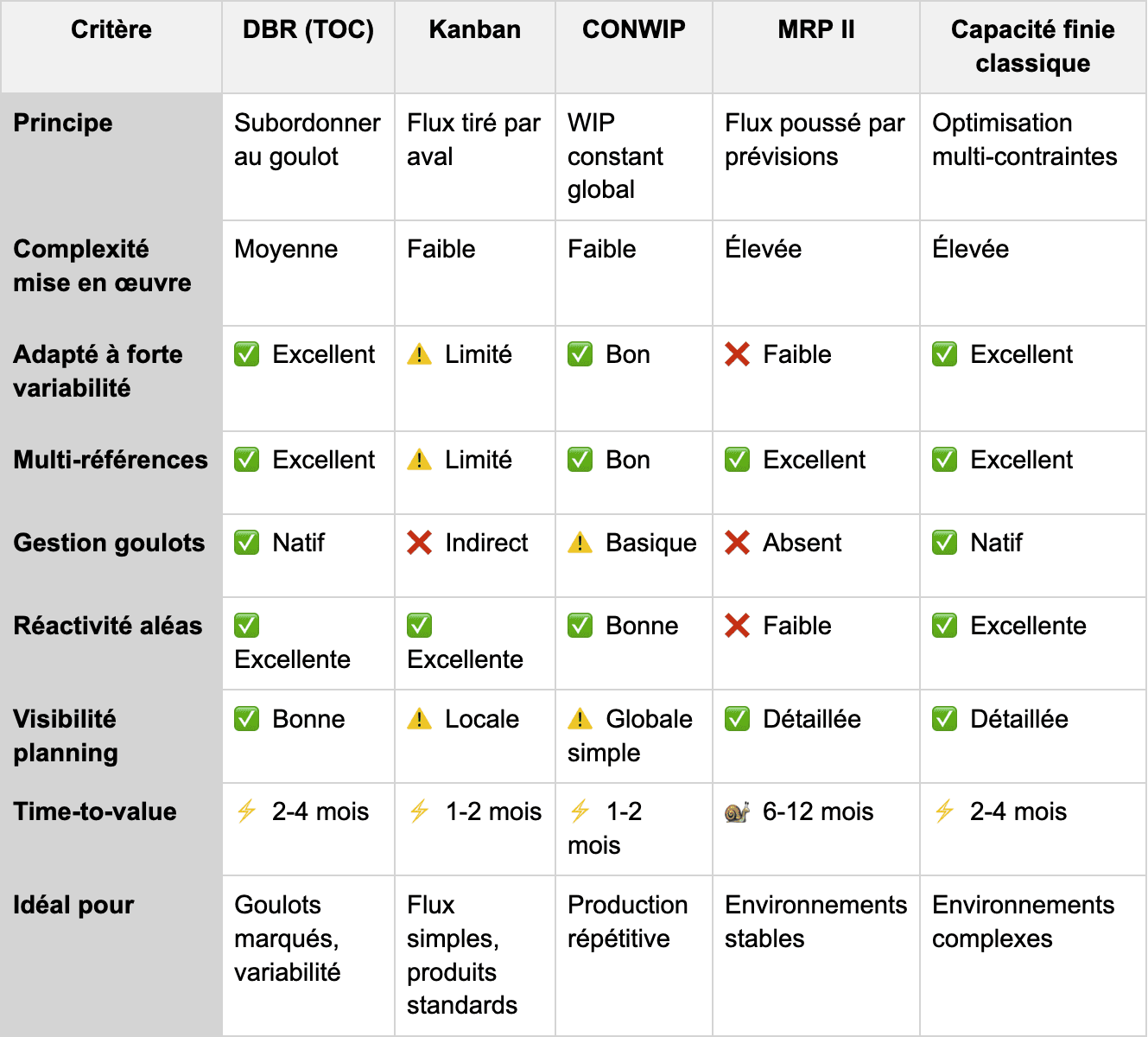
DBR vs. Kanban vs. CONWIP vs. MRP II: comparison table

Let's compare DBR with other scheduling methods to clarify their respective fields of application:

DBR + finite capacity: complementarity

DBR and finite-capacity planning are not mutually exclusive but complementary:

DBR brings the philosophy of focusing on the constraint and managing flows through buffers.

Finite capacity brings the precision of multi-constraint scheduling and advanced simulation capability.

A modern finite-capacity scheduling software can incorporate the DBR principles of the Theory of Constraints while finely managing all the system's constraints.

Scheduling with Excel: useful templates and limits

A minimal Excel template for DBR

For simple environments, Excel can be enough to get started with DBR:

Bottleneck schedule: A table listing the work orders scheduled at the bottleneck with forecast start/end dates.

Buffer-tracking table: Columns (work-order reference, bottleneck need-by date, current progress, position in the buffer, color code).

Release calculations: Formulas automatically calculating the release date of each work order according to the Rope logic.

Visual dashboard: Charts showing the distribution of work orders across the green/yellow/red zones.

The limits of Excel for DBR

Beyond a certain level of complexity, Excel reveals its limits:

Multi-constraint: Excel cannot effectively manage several potential or floating bottlenecks.

Component management: Automatically checking component availability for each work order becomes unmanageable by hand.

Multi-shop: Coordinating DBR across several sites or production lines exceeds Excel's capabilities.

Dynamic simulation: Quickly testing the impact of a disruption or a decision requires tedious manual recalculations.

Integrations: Manual imports/exports from the ERP/MES generate errors and consume precious time.

The moment to switch to scheduling software

Several signals indicate that Excel is reaching its limits for your DBR implementation:

• More than 30 active work orders at the same time

• Significant variability requiring frequent rescheduling

• Several resources that are candidates for bottleneck status

• Strict customer requirements demanding fine precision

• Excel planning time exceeding 4 hours a week

• Frequent errors in calculations or data entry

Best practices and mistakes to avoid

Common mistakes in applying the Theory of Constraints

Misidentified bottleneck: Getting the constraint wrong leads to subordinating the system to the wrong pace, worsening problems rather than solving them.

Poorly sized buffers: Too short, they expose the bottleneck to stockouts; too long, they maintain excessive work-in-progress and prolonged lead times.

Uncontrolled work-order release: Continuing to release work orders "to keep resources busy" sabotages the very principle of the Rope and causes WIP to explode.

Components not handled: Implementing DBR without managing component availability leads to frequent blockages and cancels out the benefits.

Frequent changes to the bottleneck schedule: Constantly changing the bottleneck's schedule destabilizes the entire system and prevents the establishment of a stable flow.

Remedies and best practices

Data governance: Establish rigorous processes for validating the times, routings, and capacities that feed the DBR calculations.

Supply SLAs: Formal agreements with the purchasing department guaranteeing component availability within timeframes compatible with the buffers.

Stable prioritization: Define clear priority rules and follow them to maintain the stability of the bottleneck schedule.

Monthly review: Systematically check that the bottleneck has not migrated and adjust buffers and rules accordingly.

Automation: Use a finite-capacity scheduling software to automate the complex calculations and reduce errors.

Change management

Implementing DBR according to the Theory of Constraints involves a cultural change:

Involving operators: Clearly explain the DBR logic and why some resources will appear "underused" (this is normal and desirable).

Training planners: Make sure they understand the TOC philosophy and don't fall back into traditional local-optimization reflexes.

Transparent communication of the rules: Visually display the bottleneck schedule, the buffer status, and the prioritization rules.

Celebrating successes: Measure and communicate the improvements (OTD, lead time, WIP) to strengthen buy-in.

Mini use case: transforming a machining shop

Initial context

A precision-machining shop producing 80 different references on 15 machines was facing major difficulties:

• OTD at 68% (target: >90%)

• WIP representing 8 weeks of production

• Average lead times of 12 weeks

• Customer delays generating penalties and dissatisfaction

The analysis revealed that the entire shop was constantly waiting for a highly specialized 5-axis milling machine to process parts, creating significant queues.

Implementing DBR

Identifying the Drum: The 5-axis milling machine, saturated at 95% and with 3 to 4 weeks of load systematically piling up in front of it.

Sizing the Buffer: An upstream buffer of 1 week of load in front of the milling machine, guaranteeing its continuous supply despite disruptions. A shipping buffer of 2 weeks after the milling machine.

Defining the Rope: Work-order release calculated so that they arrive in front of the milling machine when it needs them according to its schedule, i.e. 5 weeks before the customer delivery date (1 week upstream buffer + 2 weeks of pre-milling operations + 2 weeks shipping buffer).

Bottleneck schedule: Scheduling the milling machine over a rolling 4-week horizon, optimized to minimize tool changes, stabilized and protected against untimely modifications.

Results after 6 months

The measured improvements confirmed the relevance of the Theory of Constraints approach:

• OTD: Improvement from 68% to 91%, exceeding the target

• WIP: Reduction from 8 weeks to 3.5 weeks of production, freeing up cash and space

• Average lead time: Decrease from 12 weeks to 5.5 weeks, improving commercial responsiveness

• Productive saturation of the milling machine: Increase from 75% to 88% of available time

Lessons learned: The key to success lay in the discipline of releasing only what the Rope dictated, despite the temptation to "keep the machines running." Visual buffer management made it possible to focus efforts on the real problems rather than on artificial emergencies.

FAQ: Frequently asked questions about DBR and the Theory of Constraints

Is DBR suitable for small, highly varied batches?

Yes, DBR is particularly suited to high-product-mix environments. Focusing on the bottleneck actually simplifies scheduling by reducing complexity: rather than optimizing 15 resources, you concentrate on 1 or 2 critical resources. Variability is absorbed by buffers sized accordingly.

How do you size a buffer correctly?

Start from a generous estimate (5-7 days of production coverage) then observe, over 4-6 weeks, the frequency of penetrations into the red zones. If penetrations are rare (<5%), gradually reduce the buffer. If they are frequent (>15%), increase it. The goal: keep red penetrations between 5-10% of the time.

Does DBR replace the ERP or the MES?

No, DBR is a scheduling method that sits on top of existing systems. The ERP continues to manage forecasts, the MPS, and supplies. The MES continues to collect execution data. DBR uses this data to schedule production effectively. A modern scheduling software incorporates DBR while interfacing with ERP and MES.

What is the difference between DBR and Kanban/CONWIP?

Kanban limits WIP locally in front of each workstation. CONWIP limits WIP globally across the system. DBR explicitly subordinates the entire system to the pace of the identified bottleneck. DBR offers more visibility into the future schedule and better manages high-variability environments with a complex product mix, whereas Kanban excels in simple, repetitive flows.

Conclusion: Turn your bottleneck into a competitive advantage

The Drum-Buffer-Rope method, based on the Theory of Constraints, offers a radically different approach to traditional scheduling. Rather than vainly trying to balance all resources or locally optimize each workstation, DBR accepts the existence of the bottleneck and makes it the synchronization point for the entire system.

This focus generates concrete, measurable benefits: a typical improvement of 20 to 40 OTD points, a 30 to 50% reduction in lead times, a 40 to 60% drop in work-in-progress. Beyond the numbers, DBR above all brings a stability and predictability that transform the customer relationship and free up managerial energy for continuous improvement rather than perpetual firefighting.

Implementation, while requiring rigor and discipline, remains accessible: identifying the bottleneck, establishing its protected schedule, sizing the protective buffers, and releasing work orders in a controlled way according to the Rope logic. For simple environments, Excel can be enough to start. Beyond a certain level of complexity, a finite-capacity scheduling software incorporating the principles of the Theory of Constraints quickly becomes essential.

Is your bottleneck a constraint you suffer, or a performance lever you control?

🎯 Take part in our 30-minute diagnostic workshop: Identify your true bottleneck, assess your current buffers (even if they are implicit), and discover the improvement potential of your system.

📊 Request an Oplit demo to concretely see how a modern scheduling software can implement DBR in your specific environment, with simulation on your real data.